Graphics¶

Draw visualizations, microcharts, sparklines, and other data graphics.

Introduction¶

Nitro includes graphics primitives that can be composited together to create custom visualizations and charts that aesthetically match the surrounding page layout.

Graphics in Nitro are responsive, which means they resize automatically when the page size changes. Unlike SVG graphics, which resize physically, Nitro's graphics resize semantically (or logically). For example, if the points in a scatterplot are 10px wide in a visualization, they'll continue to be 10px wide when resized, so that the points do not appear distorted or skewed at different sizes.

Graphics are styled using style=, similar to how everything else is styled in Nitro.

Graphics primitives include lines, bars, points, guides, labels, and so on, covered in detail in the following sections. Each primitive is rendered using normalized coordinates (floats between 0 and 1), supplied with data=. X-values are mapped from left (0) to right (1). Y-values are mapped from bottom (0) to top (1).

Graphics primitives can be stacked to form sophisticated visualizations. To stack graphics, use the relative style on the parent box, with absolute inset-0 on each child box. This makes the boxes render on top of each other instead of one below the other.

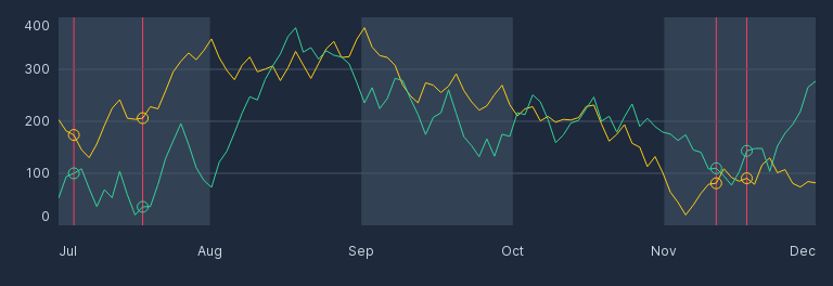
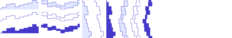
Here's a rather complicated example that creates a custom time series chart from primitives. Note that this example is just for demonstrating how compositing works, and most of the time, the graphics you create in Nitro would be significantly simpler.

# Some pretty random data:
n = 100
data1 = h2o_nitro.graphics.random_walk(n)
data2 = h2o_nitro.graphics.random_walk(n)
# Select a few random points to highlight:
highlighted = [random.randint(0, n - 1) for _ in range(4)]
guides = [i / (n - 1) for i in highlighted]
points1 = [(i / (n - 1), data1[i]) for i in highlighted]
points2 = [(i / (n - 1), data2[i]) for i in highlighted]

# Compose graphics:
layer = box() / 'absolute inset-0'
view(
    row(
        # Y-axis:
        box(
            mode='g-label',
            data=[
                # All labels are right-justified
                [1, 0 / 4, '0', 1, 0],  # first label, align top
                [1, 1 / 4, '100', 1],
                [1, 2 / 4, '200', 1],
                [1, 3 / 4, '300', 1],
                [1, 4 / 4, '400', 1, 1],  # last label, align bottom
            ],
        ) / 'w-8 h-48 text-xs text-slate-300',
        col(
            box(
                # Month shading:
                layer(mode='g-rect', data=[
                    [1 / 10, .5, 1 / 5, 1],
                    [5 / 10, .5, 1 / 5, 1],
                    [9 / 10, .5, 1 / 5, 1],
                ]) / 'fill-slate-700 stroke-none',
                # X-guides
                layer(mode='g-guide-x', data=guides) / 'stroke-rose-500 fill-none',
                # Y-guides
                layer(mode='g-guide-y', data=[.25, .5, .75]) / 'stroke-slate-600 fill-none',
                # Time-series
                layer(mode='g-line-y', data=data1) / 'stroke-yellow-400 fill-none',
                layer(mode='g-line-y', data=data2) / 'stroke-emerald-400 fill-none',
                # Highlighted points:
                layer(mode='g-point', data=points1) / 'stroke-yellow-400 fill-none',
                layer(mode='g-point', data=points2) / 'stroke-emerald-400 fill-none',
            ) / 'relative w-full h-48',
            # X-axis:
            box(
                mode='g-label',
                data=[
                    [0 / 5, .5, 'Jul', 0],  # first label, left-justify
                    [1 / 5, .5, 'Aug'],
                    [2 / 5, .5, 'Sep'],
                    [3 / 5, .5, 'Oct'],
                    [4 / 5, .5, 'Nov'],
                    [5 / 5, .5, 'Dec', 1],  # last label, right-justify
                ],
            ) / 'w-full h-8 text-xs text-slate-300',
        ) / 'w-full',
    ) / 'bg-slate-800 p-4',
)

Screenshot

Point¶

Set mode='g-point' to draw shapes at multiple points.

Set data= to a sequence of normalized [x, y, size, shape] values, where:

(x, y) is the anchor point of the shape.
size determines the size of the shape, in pixels (note that this is a fixed size, not normalized).
shape is one of c (circle, default), s (square), d (diamond), tu (triangle-up), tr (triangle-right), td (triangle-down), tl (triangle-left), h (horizontal bar), v (vertical bar), p (plus),x (cross), au (arrow-up), ar (arrow-right), al (arrow-left), ad (arrow-down).

view(
    box(
        mode='g-point',
        style='w-64 h-8 fill-none stroke-indigo-700',
        data=[
            [1 / 16, .5, 10, 'c'],  # circle
            [2 / 16, .5, 10, 's'],  # square
            [3 / 16, .5, 10, 'd'],  # diamond
            [4 / 16, .5, 10, 'tu'],  # triangle-up
            [5 / 16, .5, 10, 'tr'],  # triangle-right
            [6 / 16, .5, 10, 'td'],  # triangle-down
            [7 / 16, .5, 10, 'tl'],  # triangle-left
            [8 / 16, .5, 10, 'h'],  # horizontal bar
            [9 / 16, .5, 10, 'v'],  # vertical bar
            [10 / 16, .5, 10, 'p'],  # plus
            [11 / 16, .5, 10, 'x'],  # cross
            [12 / 16, .5, 10, 'au'],  # arrow-up
            [13 / 16, .5, 10, 'ar'],  # arrow-right
            [14 / 16, .5, 10, 'ad'],  # arrow-down
            [15 / 16, .5, 10, 'al'],  # arrow-left
        ],
    )
)

Screenshot

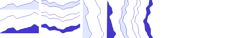
Line¶

Set mode='g-line-x' or mode='g-line-y' to draw line and area charts.

For a single line, set data= to a sequence of normalized values.

For intervals (dual lines), set data= to a sequence of normalized [low, high] values.

data = [.05, .24, .53, .61, .28, .45, .56, .68, .95, .72]
intervals = [(.62, .9), (.57, 1), (.28, .66), (.34, .77), (.25, .48),
             (0, .39), (.14, .65), (.18, .79), (.40, .78), (.61, 1)]

view(row(
    # Single curve:
    col(
        # Stroke and fill:
        box(mode='g-line-y', style='w-32 h-8 fill-indigo-100 stroke-indigo-700', data=data),
        # Stroke only:
        box(mode='g-line-y', style='w-32 h-8 fill-none stroke-indigo-700', data=data),
        # Fill only:
        box(mode='g-line-y', style='w-32 h-8 fill-indigo-700 stroke-none', data=data),
    ),
    # Dual curve:
    col(
        # Stroke and fill:
        box(mode='g-line-y', style='w-32 h-8 fill-indigo-100 stroke-indigo-700', data=intervals),
        # Stroke only:
        box(mode='g-line-y', style='w-32 h-8 fill-none stroke-indigo-700', data=intervals),
        # Fill only:
        box(mode='g-line-y', style='w-32 h-8 fill-indigo-700 stroke-none', data=intervals),
    ),
    # Single curve:
    row(
        # Stroke and fill:
        box(mode='g-line-x', style='w-8 h-32 fill-indigo-100 stroke-indigo-700', data=data),
        # Stroke only:
        box(mode='g-line-x', style='w-8 h-32 fill-none stroke-indigo-700', data=data),
        # Fill only:
        box(mode='g-line-x', style='w-8 h-32 fill-indigo-700 stroke-none', data=data),
    ),
    # Dual curve:
    row(
        # Stroke and fill:
        box(mode='g-line-x', style='w-8 h-32 fill-indigo-100 stroke-indigo-700', data=intervals),
        # Stroke only:
        box(mode='g-line-x', style='w-8 h-32 fill-none stroke-indigo-700', data=intervals),
        # Fill only:
        box(mode='g-line-x', style='w-8 h-32 fill-indigo-700 stroke-none', data=intervals),
    ),
))

Screenshot

Curve¶

Set mode='g-curve-x' or mode='g-curve-y' to draw line and area curves.

For a single curve, set data= to a sequence of normalized values.

For intervals (dual curves), set data= to a sequence of normalized [low, high] values.

data = [.05, .24, .53, .61, .28, .45, .56, .68, .95, .72]
intervals = [(.62, .9), (.57, 1), (.28, .66), (.34, .77), (.25, .48),
             (0, .39), (.14, .65), (.18, .79), (.40, .78), (.61, 1)]

view(row(
    # Single curve:
    col(
        # Stroke and fill:
        box(mode='g-curve-y', style='w-32 h-8 fill-indigo-100 stroke-indigo-700', data=data),
        # Stroke only:
        box(mode='g-curve-y', style='w-32 h-8 fill-none stroke-indigo-700', data=data),
        # Fill only:
        box(mode='g-curve-y', style='w-32 h-8 fill-indigo-700 stroke-none', data=data),
    ),
    # Dual curve:
    col(
        # Stroke and fill:
        box(mode='g-curve-y', style='w-32 h-8 fill-indigo-100 stroke-indigo-700', data=intervals),
        # Stroke only:
        box(mode='g-curve-y', style='w-32 h-8 fill-none stroke-indigo-700', data=intervals),
        # Fill only:
        box(mode='g-curve-y', style='w-32 h-8 fill-indigo-700 stroke-none', data=intervals),
    ),
    # Single curve:
    row(
        # Stroke and fill:
        box(mode='g-curve-x', style='w-8 h-32 fill-indigo-100 stroke-indigo-700', data=data),
        # Stroke only:
        box(mode='g-curve-x', style='w-8 h-32 fill-none stroke-indigo-700', data=data),
        # Fill only:
        box(mode='g-curve-x', style='w-8 h-32 fill-indigo-700 stroke-none', data=data),
    ),
    # Dual curve:
    row(
        # Stroke and fill:
        box(mode='g-curve-x', style='w-8 h-32 fill-indigo-100 stroke-indigo-700', data=intervals),
        # Stroke only:
        box(mode='g-curve-x', style='w-8 h-32 fill-none stroke-indigo-700', data=intervals),
        # Fill only:
        box(mode='g-curve-x', style='w-8 h-32 fill-indigo-700 stroke-none', data=intervals),
    ),
))

Screenshot

Step¶

Set mode='g-step-x' or mode='g-step-y' to draw step charts. Step charts are similar to line charts, except that adjacent points are connected using discrete steps instead of line segments.

For a single curve, set data= to a sequence of normalized values.

For intervals (dual curves), set data= to a sequence of normalized [low, high] values.

data = [.05, .24, .53, .61, .28, .45, .56, .68, .95, .72]
intervals = [(.62, .9), (.57, 1), (.28, .66), (.34, .77), (.25, .48),
             (0, .39), (.14, .65), (.18, .79), (.40, .78), (.61, 1)]
view(row(
    # Single curve:
    col(
        # Stroke and fill:
        box(mode='g-step-y', style='w-32 h-8 fill-indigo-100 stroke-indigo-700', data=data),
        # Stroke only:
        box(mode='g-step-y', style='w-32 h-8 fill-none stroke-indigo-700', data=data),
        # Fill only:
        box(mode='g-step-y', style='w-32 h-8 fill-indigo-700 stroke-none', data=data),
    ),
    # Dual curve:
    col(
        # Stroke and fill:
        box(mode='g-step-y', style='w-32 h-8 fill-indigo-100 stroke-indigo-700', data=intervals),
        # Stroke only:
        box(mode='g-step-y', style='w-32 h-8 fill-none stroke-indigo-700', data=intervals),
        # Fill only:
        box(mode='g-step-y', style='w-32 h-8 fill-indigo-700 stroke-none', data=intervals),
    ),
    # Single curve:
    row(
        # Stroke and fill:
        box(mode='g-step-x', style='w-8 h-32 fill-indigo-100 stroke-indigo-700', data=data),
        # Stroke only:
        box(mode='g-step-x', style='w-8 h-32 fill-none stroke-indigo-700', data=data),
        # Fill only:
        box(mode='g-step-x', style='w-8 h-32 fill-indigo-700 stroke-none', data=data),
    ),
    # Dual curve:
    row(
        # Stroke and fill:
        box(mode='g-step-x', style='w-8 h-32 fill-indigo-100 stroke-indigo-700', data=intervals),
        # Stroke only:
        box(mode='g-step-x', style='w-8 h-32 fill-none stroke-indigo-700', data=intervals),
        # Fill only:
        box(mode='g-step-x', style='w-8 h-32 fill-indigo-700 stroke-none', data=intervals),
    ),
))

Screenshot

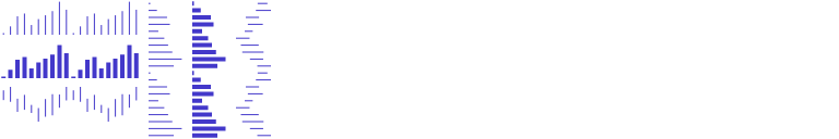
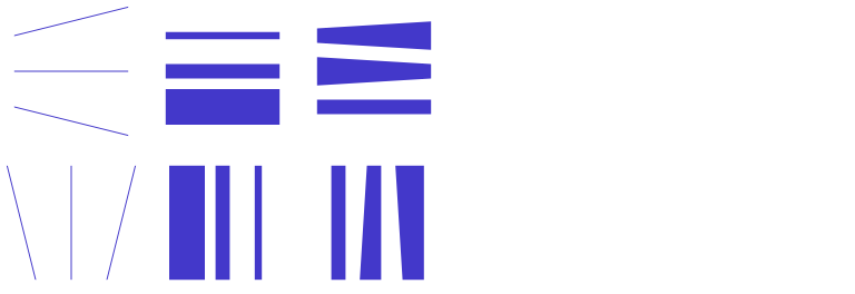
Bar¶

Set mode='g-bar-x' or mode='g-bar-y' to draw bar/column charts.

For simple bars, set data= to a sequence of normalized values.

For interval-valued bars, set data= to a sequence of normalized [low, high] values.

data = [.05, .24, .53, .61, .28, .45, .56, .68, .95, .72]
intervals = [(.62, .9), (.57, 1), (.28, .66), (.34, .77), (.25, .48),
             (0, .39), (.14, .65), (.18, .79), (.40, .78), (.61, 1)]
view(row(
    col(
        # "Column chart":
        box(mode='g-bar-y', style='w-32 h-16 stroke-indigo-700', data=data),
        # Interval-valued:
        box(mode='g-bar-y', style='w-32 h-16 stroke-indigo-700', data=intervals),
    ),
    row(
        # "Bar chart":
        box(mode='g-bar-x', style='w-16 h-32 stroke-indigo-700', data=data),
        # Interval-valued:
        box(mode='g-bar-x', style='w-16 h-32 stroke-indigo-700', data=intervals),
    )
))

Screenshot

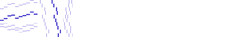
Stroke¶

Set mode='g-stroke-x' or mode='g-stroke-y' to draw a sequence of strokes. The stroke- mode is similar to the bar- mode, except that you can control the thickness of the strokes (bars) when using the stroke- mode.

For simple strokes, set data= to a sequence of normalized values.

For interval-valued strokes, set data= to a sequence of normalized [low, high] values.

data = [.05, .24, .53, .61, .28, .45, .56, .68, .95, .72] * 2
intervals = [(.62, .9), (.57, 1), (.28, .66), (.34, .77), (.25, .48),
             (0, .39), (.14, .65), (.18, .79), (.40, .78), (.61, 1)] * 2
view(row(
    col(
        # Strokes:
        box(mode='g-stroke-y', style='w-32 h-8 stroke-indigo-700', data=data),
        # Thicker strokes:
        box(mode='g-stroke-y', style='w-32 h-8 stroke-indigo-700 stroke-4', data=data),
        # Interval-valued:
        box(mode='g-stroke-y', style='w-32 h-8 stroke-indigo-700', data=intervals),
    ),
    row(
        # Strokes:
        box(mode='g-stroke-x', style='w-8 h-32 stroke-indigo-700', data=data),
        # Thicker strokes:
        box(mode='g-stroke-x', style='w-8 h-32 stroke-indigo-700 stroke-4', data=data),
        # Interval-valued:
        box(mode='g-stroke-x', style='w-8 h-32 stroke-indigo-700', data=intervals),
    )
))

Screenshot

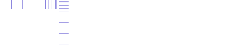
Tick¶

Set mode='g-tick-x' or mode='g-tick-y' to draw a sequence of ticks. The tick- mode is similar to the bar- mode, except that only the tip of the bar is drawn.

For simple ticks, set data= to a sequence of normalized values.

For interval-valued ticks, set data= to a sequence of normalized [low, high] values.

data = [.05, .24, .53, .61, .28, .45, .56, .68, .95, .72]
intervals = [(.62, .9), (.57, 1), (.28, .66), (.34, .77), (.25, .48),
             (0, .39), (.14, .65), (.18, .79), (.40, .78), (.61, 1)]
view(row(
    col(
        # Strokes:
        box(mode='g-tick-y', style='w-32 h-8 stroke-indigo-700', data=data),
        # Thicker strokes:
        box(mode='g-tick-y', style='w-32 h-8 stroke-indigo-700 stroke-4', data=data),
        # Interval-valued:
        box(mode='g-tick-y', style='w-32 h-8 stroke-indigo-700', data=intervals),
    ),
    row(
        # Strokes:
        box(mode='g-tick-x', style='w-8 h-32 stroke-indigo-700', data=data),
        # Thicker strokes:
        box(mode='g-tick-x', style='w-8 h-32 stroke-indigo-700 stroke-4', data=data),
        # Interval-valued:
        box(mode='g-tick-x', style='w-8 h-32 stroke-indigo-700', data=intervals),
    )
))

Screenshot

Guide¶

Set mode='g-guide-x' or mode='g-guide-y' to draw a sequence of guide lines.

Set data= to a sequence of normalized x- or y- coordinates.

view(row(
    box(
        mode='g-guide-x',
        style='w-48 h-8 stroke-indigo-700',
        data=[0, .2, .4, .6, .8, .85, .9, .95, .975, 1],
    ),
    box(
        mode='g-guide-y',
        style='w-8 h-48 stroke-indigo-700',
        data=[0, .2, .4, .6, .8, .85, .9, .95, .975, 1],
    ),
))

Screenshot

Gauge¶

Set mode='g-gauge-x' or mode='g-gauge-y' to draw a gauge.

Set data= to normalized [length, width] values:

length defines the length of the bar.
width defines the thickness of the bar relative to the track, and defaults to 1 (bar is as thick as the track).

view(row(
    col(
        box(
            mode='g-gauge-x',
            style='w-48 h-4 fill-indigo-100 stroke-indigo-700',
            data=[.75],
        ),
        box(
            mode='g-gauge-x',
            style='w-48 h-4 fill-indigo-100 stroke-indigo-700',
            data=[.75, .5],
        ),  # thinner bar
    ),
    box(
        mode='g-gauge-y',
        style='w-4 h-48 fill-indigo-100 stroke-indigo-700',
        data=[.75],
    ),
    box(
        mode='g-gauge-y',
        style='w-4 h-48 fill-indigo-100 stroke-indigo-700',
        data=[.75, .5],
    ),  # thinner bar
))

Screenshot

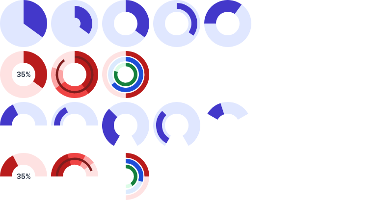
Circular Gauge¶

Set mode='g-gauge-c' to draw a circular gauge.

Set data= to normalized [length, width, track-length, track-width, rotation, diameter] values:

length is the length of the gauge bar.
width is the thickness of the gauge bar (optional, default 1).
track-length is the length of the track (optional, default 1).
track-width is the thickness of the track (optional, default 1).
rotation is the angle of rotation (optional, default 0).
diameter is the diameter of the gauge (optional, default 1).

style = 'w-24 h-24 fill-indigo-100 stroke-indigo-700'
view(
    row(
        box(mode='g-gauge-c', style=style, data=[.35]),
        box(mode='g-gauge-c', style=style, data=[.35, .5]),  # thinner bar
        box(mode='g-gauge-c', style=style, data=[.35, 1, 1, .5]),  # thinner track
        box(mode='g-gauge-c', style=style, data=[.35, .5, 1, .5]),  # thinner track and bar
        box(mode='g-gauge-c', style=style, data=[.35, 1, 1, .5, .75]),  # rotate 270 degrees
    ),
    row(
        # With label:
        box(
            box(mode='g-gauge-c', data=[.35, 1, 1, .5]) / 'absolute inset-0 fill-red-100 stroke-red-700',
            box('35%') / 'text-sm font-bold',
        ) / 'relative flex w-24 h-24 justify-center items-center',
        # Stacked:
        box(
            box(mode='g-gauge-c', data=[.8, 1, 1, .5]) / 'absolute inset-0 fill-red-100 stroke-red-300',
            box(mode='g-gauge-c', data=[.65, 1, 1, .5]) / 'absolute inset-0 fill-none stroke-red-500',
            box(mode='g-gauge-c', data=[.4, 1, 1, .5]) / 'absolute inset-0 fill-none stroke-red-700',
            box(mode='g-gauge-c', data=[.9, .2, 1, .5]) / 'absolute inset-0 fill-none stroke-red-900',
        ) / 'relative w-24 h-24',
        # Concentric:
        box(
            box(mode='g-gauge-c', data=[.5, 1, 1, .2, 0]) / 'absolute inset-0 fill-red-100 stroke-red-700',
            box(mode='g-gauge-c', data=[.65, 1, 1, .25, 0, .75]) / 'absolute inset-0 fill-blue-100 stroke-blue-700',
            box(mode='g-gauge-c', data=[.8, 1, 1, .3, 0, .5]) / 'absolute inset-0 fill-green-100 stroke-green-700',
        ) / 'relative w-24 h-24',
    ),
    row(
        box(mode='g-gauge-c', style=style, data=[.35, 1, .5, .5, .75]),
        box(mode='g-gauge-c', style=style, data=[.35, .5, .5, .5, .75]),
        box(mode='g-gauge-c', style=style, data=[.35, 1, 10 / 12, .5, 7 / 12]),
        box(mode='g-gauge-c', style=style, data=[.35, .5, 10 / 12, .5, 7 / 12]),
        box(mode='g-gauge-c', style=style, data=[.35, 1, 4 / 12, .5, 10 / 12]),
    ),
    row(
        # With label:
        box(
            box(mode='g-gauge-c', data=[.35, 1, .5, .5, .75]) / 'absolute inset-0 fill-red-100 stroke-red-700',
            box('35%') / 'text-sm font-bold',
        ) / 'relative flex w-24 h-24 justify-center items-center',
        # Stacked:
        box(
            box(mode='g-gauge-c', data=[.8, 1, .5, .5, .75]) / 'absolute inset-0 fill-red-100 stroke-red-300',
            box(mode='g-gauge-c', data=[.65, 1, .5, .5, .75]) / 'absolute inset-0 fill-none stroke-red-500',
            box(mode='g-gauge-c', data=[.4, 1, .5, .5, .75]) / 'absolute inset-0 fill-none stroke-red-700',
            box(mode='g-gauge-c', data=[.9, .2, .5, .5, .75]) / 'absolute inset-0 fill-none stroke-red-900',
        ) / 'relative w-24 h-24',
        # Concentric:
        box(
            box(mode='g-gauge-c', data=[.5, 1, .5, .2, 0]) / 'absolute inset-0 fill-red-100 stroke-red-700',
            box(mode='g-gauge-c', data=[.6, 1, .5, .25, 0, .75]) / 'absolute inset-0 fill-blue-100 stroke-blue-700',
            box(mode='g-gauge-c', data=[.8, 1, .5, .3, 0, .5]) / 'absolute inset-0 fill-green-100 stroke-green-700',
        ) / 'relative w-24 h-24',
    ),
)

Screenshot

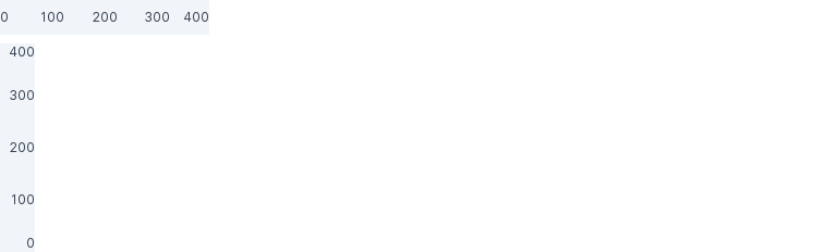
Label¶

Set mode='g-label' to draw a sequence of labels.

Set data= to a sequence of normalized [x, y, text, justify, align] values.

justify and align define the anchor point of the label:

Set justify to 0 (left), 1 (right), or .5 to center horizontally (default).
Set align to 0 (top), 1 (bottom), or .5 to center vertically (default).

view(
    box(
        mode='g-label',
        style='w-48 h-8 text-xs bg-slate-100',
        data=[
            [0, .5, '0', 0],  # first label, left-justify
            [.25, .5, '100'],
            [.5, .5, '200'],
            [.75, .5, '300'],
            [1, .5, '400', 1],  # last label, right-justify
        ],
    ),
    box(
        mode='g-label',
        style='w-8 h-48 text-xs bg-slate-100',
        data=[
            # All labels are right-justified
            [1, 0, '0', 1, 0],  # first label, align top
            [1, .25, '100', 1],
            [1, .5, '200', 1],
            [1, .75, '300', 1],
            [1, 1, '400', 1, 1],  # last label, align bottom
        ],
    ),
)

Screenshot

Rectangle¶

Set mode='g-rect' to draw multiple rectangles.

Set data= to a sequence of normalized [x, y, width, height, corner-radius] values, where:

(x, y) defines the center of the rectangle.
width and height define the size of the rectangle.
corner-radius (optional) is the corner radius in pixels (not normalized).

view(
    box(
        mode='g-rect',
        style='w-32 h-16 fill-indigo-100 stroke-indigo-700',
        data=[
            [.25, .5, .2, .9],
            [.5, .5, .2, .5],
            [.75, .5, .2, .9, 10],
        ],
    ),
)

Screenshot

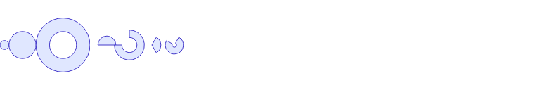
Arc¶

Set mode='g-arc' to draw multiple arcs or circles.

Set data= to a sequence of normalized [x, y, diameter, length, width, rotation] values, where:

(x, y) defines the center of the arc.
diameter defines the diameter of the arc.
length defines the length of the arc (1 for circles, fractions for arcs).
width defines the thickness of the arc (1 for discs, fractions for donuts).
rotation defines the rotation angle of the arc (.25 for 90 degrees, .5 for 180 degrees, and so on).

view(row(
    box(
        mode='g-arc',
        style='w-32 h-32 fill-indigo-100 stroke-indigo-700',
        data=[
            [.05, .5, .1],
            [.25, .5, .3],
            [.7, .5, .6, 1, .5],  # donut
        ],
    ),
    box(
        mode='g-arc',
        style='w-32 h-32 fill-indigo-100 stroke-indigo-700',
        data=[
            [1 / 8, .5, 1 / 5, 1 / 2, 1, 3 / 4],
            [3 / 8, .5, 1 / 3, 3 / 4, .5, 0],
            [5 / 8, .5, 1 / 5, 4 / 12, 1, 1 / 12],
            [7 / 8, .5, 1 / 5, 3 / 4, .75, 1 / 12],
        ],
    ),
))

Screenshot

Polyline¶

Set mode='g-polyline' to draw multiple polylines.

Set data= to a sequence of normalized [x1, y1, x2, y2, x3, y3, ...] values where xi, yi represent vertices.

view(
    box(
        mode='g-polyline',
        style='w-32 h-8 fill-none stroke-indigo-700',
        data=[
            [
                .1, .1, .1, .9,
                .2, .1, .2, .9,
                .3, .1, .3, .9,
                .4, .1, .4, .9,
                .5, .1, .5, .9,
            ],
            [
                .6, .1, .9, .1,
                .6, .3, .9, .3,
                .6, .5, .9, .5,
                .6, .7, .9, .7,
                .6, .9, .9, .9,
            ],
        ],
    ),
)

Screenshot

Polygon¶

Set mode='g-polygon' to draw multiple polygons.

Set data= to a sequence of normalized [x1, y1, x2, y2, x3, y3, ...] values where xi, yi represent vertices.

view(
    box(
        mode='g-polygon',
        style='w-32 h-8 fill-indigo-100 stroke-indigo-700',
        data=[
            [
                .1, .05, .1, .9,
                .2, .1, .2, .9,
                .3, .1, .3, .9,
                .4, .1, .4, .9,
                .5, .05
            ],
            [
                .55, .1, .9, .1,
                .6, .3, .9, .3,
                .6, .5, .9, .5,
                .6, .7, .9, .7,
                .55, .9
            ],
        ],
    ),
)

Screenshot

Link¶

Set mode='g-link-x' or mode='g-link-y' to draw connecting lines between pairs of points. Use g-link-x mode to make horizontal connections, and g-link-y to make vertical connections.

Set data= to a sequence of normalized [x1, y1, x2, y2, t1, t2] values, where:

(x1, y1) is the start point.
(x2, y2) is the end point.
t1 (optional) is the start thickness. If omitted, the stroke thickness can be controlled using style=.
t2 (optional) is the end thickness. Defaults to t1 if omitted.

view(
    row(
        box(
            mode='g-link-x',
            style='h-32 w-32 fill-none stroke-indigo-700',
            data=[
                [.1, .75, .9, .95],
                [.1, .5, .9, .5],
                [.1, .25, .9, .05],
            ],
        ),
        box(
            mode='g-link-x',
            style='h-32 w-32 fill-indigo-700 stroke-none',
            data=[
                [.1, .75, .9, .75, .05],  # add thickness
                [.1, .5, .9, .5, .1],  # more thickness
                [.1, .25, .9, .25, .25],  # even more thickness
            ],
        ),
        box(
            mode='g-link-x',
            style='h-32 w-32 fill-indigo-700 stroke-none',
            data=[
                [.1, .75, .9, .75, .1, .2],  # start thin, end thick
                [.1, .5, .9, .5, .2, .1],  # start thick, end thin
                [.1, .25, .9, .25, .1, .1],  # uniform thickness
            ],
        ),
    ),
    row(
        box(
            mode='g-link-y',
            style='h-32 w-32 fill-none stroke-indigo-700',
            data=[
                [.75, .1, .95, .9],
                [.5, .1, .5, .9],
                [.25, .1, .05, .9],
            ],
        ),
        box(
            mode='g-link-y',
            style='h-32 w-32 fill-indigo-700 stroke-none',
            data=[
                [.75, .1, .75, .9, .05],  # add thickness
                [.5, .1, .5, .9, .1],  # more thickness
                [.25, .1, .25, .9, .25],  # even more thickness
            ],
        ),
        box(
            mode='g-link-y',
            style='h-32 w-32 fill-indigo-700 stroke-none',
            data=[
                [.75, .1, .75, .9, .1, .2],  # start thin, end thick
                [.5, .1, .5, .9, .2, .1],  # start thick, end thin
                [.25, .1, .25, .9, .1, .1],  # uniform thickness
            ],
        ),
    ),
)

Screenshot

Spline¶

Set mode='g-spline-x' mode='g-spline-y' to draw connecting splines (bezier curves) between pairs of points.

Set data= to a sequence of normalized [x1, y1, x2, y2, t1, t2] values, where:

(x1, y1) is the start point.
(x2, y2) is the end point.
t1 (optional) is the start thickness. If omitted, the stroke thickness can be controlled using style=.
t2 (optional) is the end thickness. Defaults to t1 if omitted.

view(
    row(
        box(
            mode='g-spline-x',
            style='h-32 w-32 fill-none stroke-indigo-700',
            data=[
                [.1, .75, .9, .95],
                [.1, .5, .9, .5],
                [.1, .25, .9, .05],
            ],
        ),
        box(
            mode='g-spline-x',
            style='h-32 w-32 fill-indigo-700 stroke-none',
            data=[
                [.1, .75, .9, .95, .05],  # add thickness
                [.1, .65, .9, .65, .1],  # more thickness
                [.1, .45, .9, .25, .25],  # even more thickness
            ],
        ),
        box(
            mode='g-spline-x',
            style='h-32 w-32 fill-indigo-700 stroke-none',
            data=[
                [.1, .75, .9, .65, .05, .25],  # variable thickness
                [.1, .65, .9, .45, .1, .1],  # uniform thickness
                [.1, .45, .9, .35, .25, .05],  # variable thickness
            ],
        ),
    ),
    row(
        box(
            mode='g-spline-y',
            style='h-32 w-32 fill-none stroke-indigo-700',
            data=[
                [.75, .1, .95, .9],
                [.5, .1, .5, .9],
                [.25, .1, .05, .9],
            ],
        ),
        box(
            mode='g-spline-y',
            style='h-32 w-32 fill-indigo-700 stroke-none',
            data=[
                [.75, .1, .95, .9, .05],  # add thickness
                [.65, .1, .65, .9, .1],  # more thickness
                [.45, .1, .25, .9, .25],  # even more thickness
            ],
        ),
        box(
            mode='g-spline-y',
            style='h-32 w-32 fill-indigo-700 stroke-none',
            data=[
                [.75, .1, .65, .9, .05, .25],  # variable thickness
                [.65, .1, .45, .9, .1, .1],  # uniform thickness
                [.45, .1, .35, .9, .25, .05],  # variable thickness
            ],
        ),
    )
)

Screenshot

Win Loss¶

Stack two bar graphics vertically to create a win-loss graphic.

wins = [1, 0, 0, 1, 0, 1, 1, 1, 0, 0, 0, 0, 1, 1, 1, 0, 0, 1] * 2
losses = [(x + 1) % 2 for x in wins]  # invert wins
view(
    box(
        box(mode='g-bar-y', style='w-48 h-4 stroke-green-700', data=wins),
        box(mode='g-bar-y', style='w-48 h-4 stroke-red-700', data=losses),
    )
)

Screenshot

Stacked bar¶

Overlay multiple gauges to create a stacked bar.

bar = box(mode='g-gauge-x') / 'absolute inset-0 fill-none'
view(
    box(
        bar(data=[1.0]) / 'stroke-green-400',
        bar(data=[.8]) / 'stroke-lime-400',
        bar(data=[.7]) / 'stroke-amber-400',
        bar(data=[.3]) / 'stroke-orange-400',
        bar(data=[.1]) / 'stroke-red-400',
    ) / 'relative w-48 h-4',
)

Screenshot

Bullet graph¶

Overlay multiple gauge and guide graphics to create a bullet graph.

layer = box() / 'absolute inset-0 fill-none'
gauge = layer(mode='g-gauge-x')
view(
    row(
        box(
            box('Revenue') / 'font-medium text-sm',
            box('U.S. $(1,000s)') / 'text-xs'
        ) / 'text-right',
        box(
            box(
                gauge(data=[1]) / 'stroke-slate-200',  # band
                gauge(data=[.8]) / 'stroke-slate-300',  # band
                gauge(data=[.6]) / 'stroke-slate-400',  # band
                gauge(data=[.7, .25]) / 'stroke-slate-900',  # measure
                layer(mode='g-guide-x', data=[.9]) / 'stroke-red-800',  # reference
            ) / 'relative w-48 h-6',
            box(
                mode='g-guide-x', data=[i / 6 for i in range(0, 7)]
            ) / 'w-48 h-1 stroke-slate-800',
            box(
                mode='g-label', data=[(i / 6, 0, str(i * 50)) for i in range(0, 7)]
            ) / 'w-48 h-2 text-xs',
        ) / 'flex flex-col'
    )
)

Screenshot

Sankey diagram¶

Overlay splines to create a sankey diagram.

n_src, n_dst = 3, 9  # number of sources and destinations
whitespace = .5
domain = [[random.random() for _ in range(n_dst)] for _ in range(n_src)]  # fake data

# Normalize domain, minus whitespace:
dsum = sum([sum(ds) for ds in domain])  # sum
range_ = [[d * whitespace / dsum for d in ds] for ds in domain]

# Compute spacing between bunches
dy1, dy2 = (1 - whitespace) / n_src, (1 - whitespace) / n_dst
x1, y1, x2, y2 = 0, dy1 / 2, 1, dy2 / 2

bunches = []
# Pass 1: Compute start positions
for rs in range_:
    bunch = []
    for r in rs:
        edge = [x1, y1 + r / 2, x2, y2, r]
        bunch.append(edge)
        y1 += r
    y1 += dy1  # spacing
    bunches.append(bunch)

# Pass 2: Compute end positions
for j in range(n_dst):
    for i in range(n_src):
        edge = bunches[i][j]  # (x1, y1, x2, y2, r)
        r = edge[4]
        edge[3] = y2 + r / 2
        y2 += r
    y2 += dy2  # spacing

# Now the simple part: render splines
splines = box(mode='g-spline-x') / 'absolute inset-0 stroke-none'
colors = [f'fill-{color}-300' for color in ['amber', 'rose', 'sky']]
view(
    box(
        *[(splines(data=bunch) / colors[i]) for i, bunch in enumerate(bunches)]
    ) / 'relative w-full h-96'
)

Screenshot

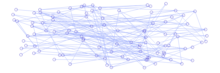
Network graph¶

Overlay point and link graphics to create a network graph (node-link diagram).

n = 100
nodes = [(random.uniform(.05, .95), random.uniform(.05, .95)) for _ in range(n)]
edges = []
for x1, y1 in nodes:
    for x2, y2 in random.choices(nodes, k=random.randint(1, 2)):
        edges.append((x1, y1, x2, y2))

layer = box() / 'absolute inset-0'
view(
    box(
        layer(mode='g-link-x', data=edges) / 'stroke-indigo-300 fill-none',
        layer(mode='g-point', data=nodes) / 'stroke-indigo-700 fill-none',
    ) / 'relative h-64',
)

Screenshot